8. Multiplier-Accelerator Interaction theory
The Keynesians have attempted to explain the business cycles in terms of the multiplier.
According to the multiplier theory, changes in investment cause multiple changes in the level of income and employment, thus deepening a depression or heightening a boom. However, the theory is unable to explain the cyclical nature of a business cycle.
According to the accelerator theory, the current level of investment is positively related to the expected rate of growth of the GDP.
According to J. R. Hicks and Professor Samuelson, the different phases of a business cycle can be explained in terms of the interaction between the accelerator and the multiplier.
While the multiplier shows how changes in investment cause multiple changes in the level of income and employment, the accelerator shows how the current level of investment is positively related to the expected rate of growth of the GDP.
Samuelson’s Model
Samuelson’s model is regarded as the first step in the direction of integrating theory of multiplier and the principal of acceleration in the attempts to explain business cycles. His model shows how multiplier and acceleration interact with one other to generate additional income, consumption and investment demands more than expected, and how economic fluctuations take place.
To understand Samuelson’s model, let us recall the distinction between autonomous and derived investment. Autonomous investment is the investment made due to exogenous factors such as new inventions and innovations in the technique of production, production process, discovery of new markets, etc. Derived investment is the investment which is induced by or undertaken due to decrease in the interest rate and increase in consumer demand necessitating new investment.
To describe the interaction process briefly, when autonomous investment takes place in a society, income of the people rises and the process of multiplier begins. Increase in income leads to increase in demand for consumer goods depending on the marginal propensity to consume. If there is no excess production capacity, the existing stock of capital would prove inadequate to produce consumer goods to meet the rising demand. Due to demand exceeding supply, prices of consumer goods begin to rise. Rise in prices leads to rise in profits. Rise in profits induces new investments. Thus, increase in consumption creates demand for investment—the derived investment. This makes the beginning of acceleration process. When derived investment takes place, incomes rise further, in the same manner as it happens when autonomous investment takes place. With increase in income, demand for consumer goods rises. Here the process of multiplier joins the process of acceleration. This is how the multiplier and the accelerator interact with each other and make the incomes grow at a rate much faster than expected.
In his analysis of interaction between multiplier and accelerator, Samuelson assumes:
i. no excess production capacity.
ii. one-year lag in income and consumption;
iii. one-year lag in investment and consumer demand; and
iv. no government activity and foreign trade.
Samuelson’s formal model and his conditions for economic fluctuations are presented below. Given the assumption (iv), the economy will be in equilibrium when
Yt = Ct + It (22.1)
where Yt = national income. Ct = total consumption expenditure, and It = investment expenditure, all in period t.
Given the assumption (ii), the consumption function may be expressed as
Ct = a Yt-1 (22.2)
where Yt-1 is income in period t-1, i.e., of the preceding year, and a is mpc.
Given the assumption (iii), investment function with a one-year lag with consumer demand is
expressed as
It = b(Ct – Ct-1) (22.3)
where b represents capital/output ratio (which determines accelerator).
By substituting Eq. (22.2) for C, and Eq. (22.3) for the equilibrium condition of the economy
Eq. (22.1) can be expressed as
Yt = α Yt-1 + b (Ct – Ct-1) (20.4)
If Ct = α Yt-1, then Ct-1 = α Yt-2. Putting the value of Ct-1 in the preceding equation, we get
Yt = α Yt-1 + b (α Yt-1 -α Yt-2) (20.5)
Yt = α (1 + b) Yt-1 – abYt-2 (equation for equilibrium) (20.6)
Eq. (20.6) is the final form of equilibrium equation. This equation reveals the two necessary information for analyzing the business cycles:
- that if the values for a and b, and incomes of two preceeding years are known, then income for any past or future year can be determined, and
- that the rate of variation in income would depend on the values of parameters a and b.
Samuelson has shown in his work the various kinds of cycles that would be generated by different combinations of a and b. Through a diagram reproduced in the figure 1, he has shown the various types of cycles caused by the different combinations of a and b. The various combinations of a and b have been marked by areas shown as A,B,C and D, each having a different pattern of trade cycles shown in figure 2. The various combinations of a and b and the corresponding natures of cycles may be briefly described as follows:
Figure 1 : Combinations of mpc (a) and accelerator (b) cycles
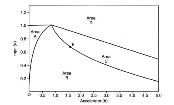
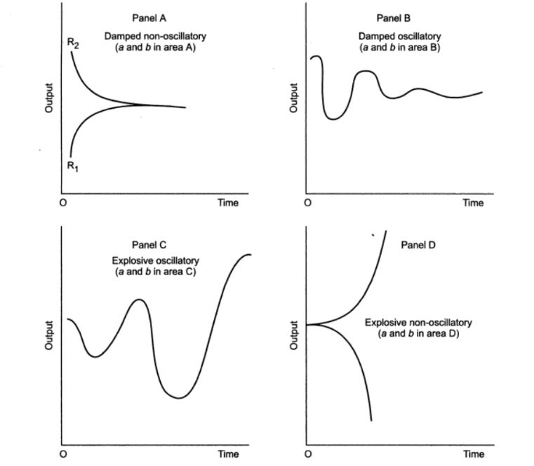
Fig. 2 Trade cycle patterns with different combinations of mpc (a) and accelerator (b)
i. Combinations of a and b in Area A produce Damped Non-oscillatory Cycles.
If all the combinations of parameters a and b fall in Area A in Fig. 1, incomes move upward or downward, depending on whether autonomous investment increases or decreases, at decreasing rates, asymptotically reaching a new equilibrium as shown in Panel A of Fig. 2. If autonomous investment increases, the economy takes route otherwise route R2.
ii. Combinations of a and b in Area B produce Damped Oscillatory Cycles
If combinations of a and b fall in Area B. it produces cycles of amplitude growing smaller and smaller until the cycles disappear and the economy ultimately stabilizes, as shown in Panel B of Fig. 2.
iii. Combinations of a and b in Area C produce Explosive Oscillatory Cycles
The combinations of a and b in Area C in Fig. 1 produce a series of trade cycles with larger and larger amplitude. This area is of explosive cycles. (See Panel C of Fig. 2)
iv. Combinations of a and b in Area D produces Explosive Aon-oscillatory Cycles
Combinations of a and b falling in Area D in Fig. 1, make the income increase (or decrease) at an exponential rate until the ceiling (or bottom) is hit (See Panel D of Fig. 2).
vi. A combination of a and b at point E produces a regular business cycle of equal amplitude. Point E shows a unique combination of a and b which produces cycles of equal amplitude that continue forever.
Criticism
Samuelson’s model is highly acclaimed as a pioneering attempt to integrate the Keynesian multiplier theory and Clark’s acceleration principle to explain business cycle. However his model is discredited for the following shortcomings.
i. Samuelson’s model is regarded by its critics as far too simple a model to fully explain what actually happens during the period of economic fluctuations. In their opinion, it is developed on highly simplifying assumptions.
ii. This model emphasizes the role of multiplier and accelerator, and interaction between them in economic fluctuations. Like many earlier theories, Samuelson’s model too leaves out or gives little consideration to many other important factors which might play an equally important role in business cycles, e.g. the role of producer’s expectations, changing psychology, changing psychology changing consumer’s preferences, and exogenous factors.
iii. One of the major shortcomings of the model is that it assumes constancy of capital/output ration whereas there is a great likelihood of changes in this ration during the periods of upswings and downswings. If this assumption is dropped, cycles may have different shapes and amplitudes from suggested by the model.
iv. As Shapiro has pointed out, many cyclic patterns suggested by the model do not conform to the real world experience.
Hicksian Theory of Trade Cycle
Hicks combines Samuelson’s multiplier-accelerator interaction model and harrod-Domar growth model to expound his theory of trade cycle. In his opinion, business cycles have historically taken place against the background of economic growth, and hence, the trade cycle theory should be linked with growth theory. In his theory of trade cycle, Hicks uses
- Keynesian concept of saving-investment relation and the multiplier
- Clark’s acceleration principle
- Samuelson’s multiplier-accelerator interaction
- growth model of Harrod and Domar
These are the main ingredients of Hick’s theory of trade cycle.
Assumptions
i. Hicks assumes an equilibrium rate of growth in the model economy in which realized growth rate (Gr) equals the natural growth rate ( Gn). The autonomous investment increases at a constant rate which always equals the rate of increase in voluntary savings . the equilibrium growth rate is determined by the rate of autonomous investment and savings.
ii. Hicks assumes a Samuelson-type of consumption function, i.e., Ct = aYt-1 (with one-year lag in consumption). The reasons he gives for the lagged consumption function are:
-
- Lag of expenditure behind income and
- Lag in non-wage income behind the change in GNP.
The saving function naturally becomes the function of past year’s income.
Given these assumptions, Hicks multiplier become a ‘mathematical truism’. With the lagged relations between income and saving-investment, the multiplier process has a dampening effect on the fluctuations. The lagged multiplier acts as ‘a depressant on upswing and a counterforce on the downswing.’.
iii. Hicks assumes that autonomous investment is a function of current output, and is undertaken to replace the wornout capital, the induced investment, in his model, is a function of change in output. The change in output generates induced investment which brings the accelerator principle in action. It may be noted here that this acceleration interacts with multiplier effect upon income and consumption.
iv. Finally, unlike Samuelson’s ever-widening, explosive cycles, Hicks prescribes ‘ceiling and bottom for the upswing and downswing. The ceiling on upward expansion is imposed by the ‘ scarcity of employment resources’. As regards the limit of the downswing, he says ‘there is no such direct limit on contraction. But an indirect limit is imposed by the mechanism of accelerator on the downswing.
Graphical Presentation of Hick’s Theory of Trade Cycle
Hicks has outline his theory of trade cycle in a diagram. The vertical axis measures the logarithms of output and employment and the horizontal axis measures time by its semi-logarithmic scale. In the diagram line AA shows the course of autonomous investment, increasing at a constant rate. The line EE is the equilibrium path of output which is a constant multiple of autonomous investment. The line FF is the full employment ceiling. The line LL shows the equilibrium path during the period of slump, assuming the output level will never go below this level.
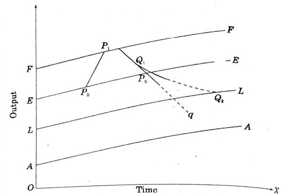
Let us suppose that economy has been progressing on the dynamic equilibrium path, and reaches point Po. Suppose also that at this juncture autonomous investment takes place due to some invention. Consequently, output increases and the economy leaves the equilibrium path EE and moves upward. After a certain lag begins the multiplier process caused by the autonomous investment. As a result, output and employment increase. Increase m output leads to induced investment which in turn brings the accelerator in action. This interaction between the multiplier and accelerator causes expansion in the economy which then moves along the expansion or oscillation pat P0P1 until point P1 is reached. The expansion beyond P1 will not be possible because of full employment constraint. The most it can do is to creep along the ceiling FF. But it cannot do so for long. For, the initial burst of autonomous investment was supposed to be short-lived; ’thus on the upper part of the path P0P1 no more than the normal amount of autonomous investment is taking place. It implies that the expansion along P0P1 has been mainly on account of the induced investment during the preceding periods.
However, once the ceiling is hit, the expansion sustained by the induced investment along FF is bound to end and a downswing becomes inevitable sooner or later. For, increase in output along FF is not high enough to induce investment and hence the induced investment ceases to take place. The downswing may be prolonged if output-investment (induced) relation has a 3 or 4 year lag. But the downfall in output is inevitable. Once the downfall has started, it must continue till it hits line EE. Since there is nothing in the process to stop it at EE, the downfall will continue further. The rate of fall , however, should be lower since the disinvestment is limited to the rate of depreciation which goes on decreasing following the decrease in output. That is, the reverse accelerator does not work as fast as it does during the upswing: there is a marked lack of symmetry. Even though the process of decline in output may be slower, a situation characterised by slump does take place in due course, Here, the autonomous investment is reduced a little below the normal level , while induced investment is zero.
The course of slump is shown by curve Q1Q2 That is, the absolute magnitude of output decreases along the curve Q1Q2 towards the slump equilibrium line LL. Another course of possible slump by Q1q, when the output plunges downward indefinitely, which is a rare possibility. The normal course of slump is Q1Q2.
Turning to recovery, when the downswing hits the bottom, it starts moving along the lower equilibrium line LL. This line is geared to the autonomous investment line AA, and rises with it. Thus, at this stage output will again have started to rise. This increase in output should bring the accelerator back into action. This marks the beginning of recovery. Once the autonomous investment starts coming in, the process of multiplier and later, its interaction with accelerator makes the economy grow on the path of expansion towards equilibrium path EE. This completes the cycle.
Criticism and Limitations
i. Hicks assumed fixed values for the multiplier and accelerator. This is unrealistic, for the values would be different during the different phases of the cycle.
ii. According to Kaldor, the weakest point in Hicks’ theory is the use of the crude acceleration principle.
iii. Duesenherry observes that the concept of ceiling in the Hicksian model is quite unnecessary for the explanation of the cycle.
iv. According to Duesenberry, the idea of the relation of the equilibrium rate of growth to the autonomous investment seems to be wrong.
v. One cannot really explain the behaviour of a cycle by the mechanical interaction of the multiplier and accelerator.
vi. According to Hansen, Hick’s free cycle idea offers a better explanation of upper turning point than the constrained cycle.
vii. The treatment of trend in the form of autonomous investment remains arbitrary.
viii. Hick’s model abstracts from many of the variables related to growth and institutional change.
ix. According to Mc Dougall and Dernberg, full employment ceiling is considered independent of the path of output. It is assumed to grow at the same rate as autonomous investment. But full employment ceiling depends on the magnitude of resources. It is also not proper to give autonomous investment a passive role.
x. Although Hicks wanted to combine trend and cycle, he could not satisfactorily do so.
xi. Hicks have attached less importance to monetary factors. He also neglected the interaction of monetary and real factors.
xii. Hicks should have perhaps given more significance to expectation and its role.
While critics have highlighted die deficiencies of Hicks’ theory, they have also highly praised his work. For example, Kaldor has referred to the “many brilliant and original pieces of analysis” found in Hicks’ theory. Duesenberry has described it as an ‘’ingenious piece of work” and “the first coherent theory of the cycle to appear in some years”. Similarly, Shapiro praises Hick’s work by saying “Hicks model remains in a sense, the last word in business cycle theory’.