3. The Non-monetary Overinvestment Theory
This theory, like Hayek’s monetary over-investment theory, states that the boom is accompanied by an excessive amount of investment and that this over-investment is the basic cause of depression. But it differs from Hayek’s theory in that it does not attach much importance to the monetary factors as causing expansion and contraction in the economy. The theory regards the money system as a part of the response mechanism in the process of business cycle, but not as a causative factor. The chief formulators of this theory are Spiethoff, Cassel and Robertson.
4. Schumpeter’s Theory of Innovation
Schumpeter’s theory of innovation falls in the line with the investment theories of business cycles. While other investment theories emphasizes the general fluctuation in investment accompanied by monetary expansion as the cause of business fluctuations. Schumpeter’s theory emphasizes innovations in business as the main cause of increase in investment and business fluctuations. By innovations he means such changes of the combination of factors of production as cannot be effected by infinitesimal steps or variations on the margin.
Innovation consists :
i. Changes in methods of production and transportation
ii. Changes in industrial organization
iii. Changes in production of new article
iv. Opening of new market or of new source of material
Innovations are nor meant by inventions which are simply the commercial application of new techniques, new materials, new means of transportation and new sources of energy. According to Schumpeterian theory, innovations are the cause of cyclical fluctuations.
Schumpeter has developed a model in two stages which he calls the first approximation and the second approximation. The first approximation deals with the initial impact of the innovatory ideas, and the second approximation deals with the subsequent waves that are created by the application of innovations.
i. The first approximation of Schumpeter’s model starts with the economic system in equilibrium in which there is no involuntary unemployment; each firm has its mc = mr and price = average cost. Also, there is no incentive for additional investment nor disincentive to reduce it. Under the conditions of complete equilibrium in the economy, if an innovation in the form of a new technique or a new process of production is introduced, it will have to be financed through bank credit. For, the economy being in equilibrium, there is no surplus fund to finance the new adventure. With additional funds available from the banking system, the innovating firms go on bidding higher prices for other inputs with a view to withdraw them from other uses. Due to increased spending in the economy, prices begin to rise. This process is further accelerated when other firms imitate the innovation and acquire additional funds from the banks. With the widespread adaptation of the innovation, output begins to flow into the market. The phase of expansion gets underway. But beyond a certain level, increased output causes decrease in price and profitability, Since further innovation do not come by quickly, there would not be additional demand for funds, Rather the firms which had earlier borrowed from the banks start paying back, This leads to contraction in money supply. Hence prices fall further. The process of recession begins and continues until equilibrium is once again restored.
ii. The second approximation of Schumpeter’s model analyses the secondary waves that are created by way of the first approximation. The main element in the secondary wave is speculation. When the primary wave of expansion begins, investors, particularly in capital goods industries, expect that the upswing is permanent. With this expectation, existing forms borrow heavily. Even consumers anticipating higher price in future go into debt to acquire durable consumer goods, investors and consumers, find it extremely difficult to meet their obligations. This situation leads to a panic and then to depression. The lower turning point comes when the necessary liquidation of assets built on borrowed funds has been completed, the debt structure has been brought to order and inefficient firms are eliminated.
Criticism
i. According to M.W. Lee an objective evaluation of Schumpeter’s theory of the cycle is not only difficult but also unavailing because much of his arguments is based on sociological rather than economic factors. Hence this theory can hardly be put to test.
ii. This theory like many other theories, leaves out many other important factors causing fluctuations. Innovation is only one of the factors and not the sole factor.
5. Psychological theory of trade cycle
The psychological theory of trade cycle was associated with the name of a classical economist A.C. Pigou. According to him, changes in the psychology of businessmen are responsible for trade cycles. When business is good, businessmen expect good profit and they feel very optimistic about future. So producers expand their business activities beyond their capacity. This leads to overproduction. Producers find it difficult to sell their products. As a result, prices fall and producers suffer losses. They become pessimistic about future. So producers curtail their business activities. Therefore, trade cycles are due to the psychological fallings of optimism and pessimism in business.
6. Under consumption theories
The under consumption theory of trade cycle was associated with the name of English economist J. A. Hobson (1858-1940). According to him, under consumption or over saving is the cause of trade cycle. When trade is good, incomes of the rich people increase greatly. They save a large part of their income and invest in the expansion of business activities. But most of the people do not have sufficient purchasing power because of low income. So producers find it very difficult to sell their products. Prices fall heavily and thus depression begins. Thus depression is caused because rich people save more and most of the people do not have enough purchasing power to buy all these products produced.
7. Cobweb model or Cobweb theory
The cobweb model or cobweb theory is an economic model that explains why prices might be subject to periodic fluctuations in certain types of markets. It describes cyclical supply and demand in a market where the amount produced must be chosen before prices are observed. Producers’ expectations about prices are assumed to be based on observations of previous prices. Nicholas Kaldor analyzed the model in 1934, coining the term “cobweb theorem”, citing previous analyses in German by Henry Schultz and Umberto Ricci. The Cobweb Theorem attempts to explain the regularly recurring cycles in the output and prices of farm products. Frankly speaking, it is not a business cycle theory for it relates only to the farming sector of the economy.
This theorem is based on three assumptions:
i. Perfect competition in which each producer assumes that present prices will continue and that his own production plans will not affect the market,
ii. Price is completely a function of the preceding period’s supply
iii. The commodity concerned is perishable. These assumptions show that the theory is particularly applicable to agricultural products.
The cobweb model is generally based on a time lag between supply and demand decisions. Agricultural markets are a context where the cobweb model might apply, since there is a lag between planting and harvesting . Suppose for example that as a result of unexpectedly bad weather, farmers go to market with an unusually small crop of strawberries. This shortage, equivalent to a leftward shift in the market’s supply curve, results in high prices. If farmers expect these high price conditions to continue, then in the following year, they will raise their production of strawberries relative to other crops. Therefore, when they go to market the supply will be high, resulting in low prices. If they then expect low prices to continue, they will decrease their production of strawberries for the next year, resulting in high prices again.
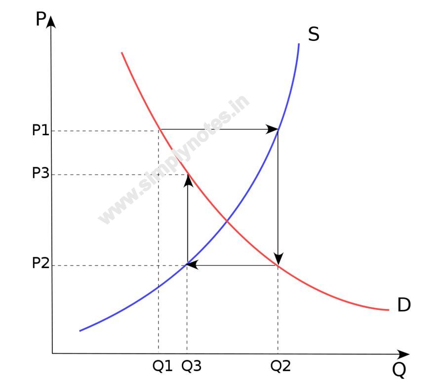
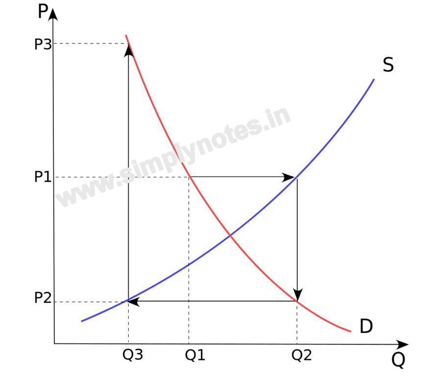
This process is illustrated by the adjacent diagrams. The equilibrium price is at the intersection of the supply and demand curves. A poor harvest in period 1 means supply falls to Q1, so that prices rise to P1. If producers plan their period 2 production under the expectation that this high price will continue, then the period 2 supply will be higher, at Q2. Prices therefore fall to P2 when they try to sell all their output. As this process repeats itself, oscillating between periods of low supply with high prices and then high supply with low prices, the price and quantity trace out a spiral. They may spiral inwards, as in the top figure, in which case the economy converges to the equilibrium where supply and demand cross; or they may spiral outwards, with the fluctuations increasing in magnitude.
The cobweb model can have two types of outcomes:
i. If the supply curve is steeper than the demand curve, then the fluctuations decrease in magnitude with each cycle, so a plot of the prices and quantities over time would look like an inward spiral, as shown in the first diagram. This is called the stable or convergent.
ii. If the slope of the supply curve is less than the absolute value of the slope of the demand curve, then the fluctuations increase in magnitude with each cycle, so that prices and quantities spiral outwards. This is called the unstable or divergent
Two other possibilities are:
i. Fluctuations may also remain of constant magnitude, so a plot of the outcomes would produce a simple rectangle, if the supply and demand curves have exactly the same slope (in absolute value).
ii. If the supply curve is less steep than the demand curve near the point where the two curves cross, but more steep when we move sufficiently far away, then prices and quantities will spiral away from the equilibrium price but will not diverge indefinitely; instead, they may converge to a limit cycle.
In either of the first two scenarios, the combination of the spiral and the supply and demand curves often looks like a cobweb, hence the name of the theory.
Limitations of Cobweb theory
Rational expectations. The model assumes farmers base next years supply purely on the previous price and assume that next year’s price will be the same as last year (adaptive expectations). However, that rarely applies in the real world. Farmers are more likely to see it as a ‘good’ year or ‘bad year and learn from price volatility.
Price divergence is unrealistic and not empirically seen. The idea that farmers only base supply on last year’s price means, in theory, prices could increasingly diverge, but farmers would learn from this and pre-empt changes in price.
It may not be easy or desirable to switch supply. A potato grower may concentrate on potatoes because that is his specialty. It is not easy to give up potatoes and take to aubergines.
Other factors affecting price. There are many other factors affecting price than a farmers decision to supply. In global markets, supply fluctuations will be minimized by the role of importing from abroad. Also, demand may vary. Also, supply can vary due to weather factors.
Buffer stock schemes. Governments or producers could band together to limit price volatility by buying surplus


